The Srivus Scientifica mark

Reimagining STEM Education: Advancing Equity Through Digital Access and Freedom

We cannot truly reimagine STEM education while essential learning tools are locked behind monthly subscriptions. Today’s pay-to-play software economy creates a quiet but devastating divide between students who have digital access and those who are left behind. Educational equity, digital access and digital freedom belong together. No child's education should depend on a recurring payment, on data they were never meant to hand over, or on permission to keep using what they were already given. If we want a more equitable society, we must build a system where the keys to the future belong to every child, not just those who can afford the recurring fee.

A scientific calculator that grows with you into a programming system. It is first a scientific calculator, and both the question and the answer stay on screen. As you grow more confident, the same system and its language, Srivus, will teach you to program, and you will never have to start over on a different tool.

Stand-alone and offline. It never needs the internet.

Free, complete, and it does not expire. Windows, macOS and Linux.
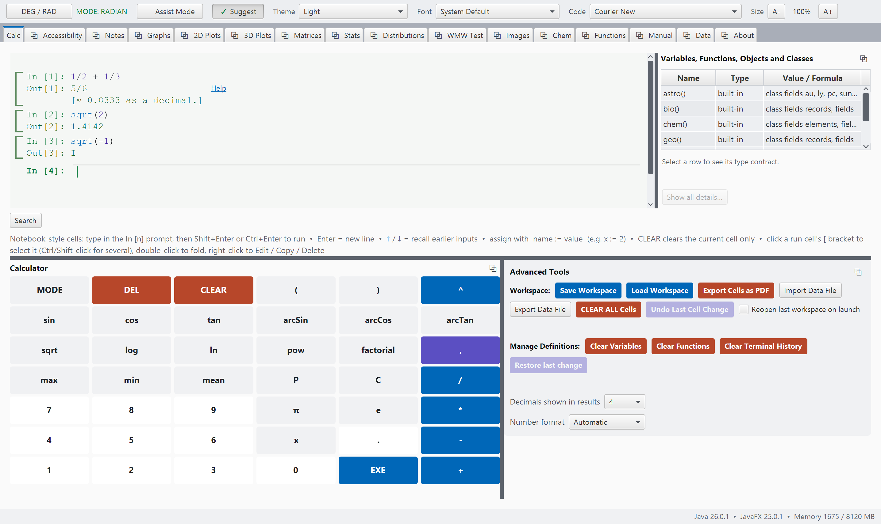
The Srivus Scientifica calculator with a worked session on screen

Why I built this

My reason for building this system is twofold.

I have always wanted to build a solid computational system for students, one that bridges the typical hand-held scientific calculators and the full-fledged computational and programming systems like Matlab, Mathematica, R, Java and Python.

The second reason is equally important, but it hits deeper in the heart. During my time as a Math teacher at a high-need charter school in Redwood City, California, a few of my students confided in me, early in the semester, that they had no internet access at home. Even though they had their school-issued Chromebooks, they could not access popular web-based learning apps while at home. This disheartening revelation weighed heavily on me. I wanted to build a system like this one for them, but I was too busy. Finally, I put everything together in the Summer of 2026 and built a stand-alone and offline desktop application, which I hope will be useful to students and teachers alike.

That is why this is a desktop application and not a website. Everything is on your own machine: the whole language, the manual, and the full reference. There is no account to create and nothing to sign in to, and once it is installed it never needs the internet again. The goal is simply to provide teachers and students with a capable educational tool while keeping access straightforward, private, and practical. I call this principle YDNB—“Your Data, Not My Business”: a zen-like approach to privacy in which the system quietly stays out of the way, allowing learning to move productively and effortlessly like the flow of a clear stream, without unnecessary collection, surveillance, or intrusion.

This system is dedicated to all students, especially my former students.

What this system is

Both the question and the answer stay on screen. You can save your work.

A typical hand-held calculator forgets. A good scientific calculator remembers only the previous answer. Here the whole conversation stays where you can see it, so you can look back over your work one step at a time the way you would in an exercise book, change one number, and run it again. Best of all, you can save your work on your computer and load it up for review at a later time!

In both editions

Whole numbers stay exact, however large

An ordinary calculator stores a number in a fixed number of binary digits, so past 2^53 it can no longer tell one whole number from the next: add 1 and the display does not change. Here whole-number arithmetic is exact, and the answer is printed in full — every digit, on the result line. Once a number runs past ten digits, a second line gives the same answer in scientific notation, as a reading aid and never a warning.

In2^53 + 1
Out9007199254740993 [≈ 9.007199254741E15 in scientific notation.]

This is the classic floating-point trap, in which adding 1 changes nothing. Here the odd number arrives intact, written out whole, with the scientific reading underneath for judging its size at a glance.

A calculator session showing exact and inexact results
In both editions

Graphs you can shade, drag and question

Students can plot curves with expressions or equations, shade regions with inequalities, and use sliders to see how changing a parameter affects these geometric objects in real time. I also designed the graphing system with accessibility in mind: different curves are distinguished not only by color, but also by distinct line and dash patterns.

A graph should also answer questions, so three readouts are built in. Trace moves along a curve and reports its coordinates; Intersect finds where two curves cross; Table of values lists the visible curve as a column of x and y. The readouts always refer to the curves on screen: change an expression and the numbers change with it.

A reading also stays on screen once you have it. You can move the pointer off the plot (to write the number down, or to reach the control beside it) and the last point you were on is still shown. It is cleared only when something that would change it changes, e.g., panning the window or editing the curve. Every plot in the program behaves this way and prints its reading at the same size, so what you learn on the Graphs tab applies to the 2D Plots, 3D Plots, Stats, Distributions and Chem plots as well.

Curve fitting is not limited to a line of best fit. Data can be fitted as a straight line, a polynomial, an exponential, a power law or a logarithm, namely linearFit, polynomialFit, exponentialFit, powerFit and logarithmicFit. Each result records which kind of curve was fitted, so the same fitValue works on any of them.

InlinearFit([1, 2, 3], [2, 4, 6])
Out["form": "linear", "slope": 2, "intercept": 0, "r": 1, "rSquared": 1, "n": 3]

The points lie exactly on y = 2x, so the slope is 2, the intercept is 0 and the fit is perfect. The result is an ordinary dictionary, so any part of it can be taken out and used.

The graph also marks the holes. A function can have no value at exactly one place, e.g., sin(x)/x at zero or (x-1)*(x+1)/(x-1) at one. Such a place is far narrower than a pixel, so the graph locates it by reading your formula. A hollow circle marks the height the curve approaches but never reaches, as a textbook draws it, and it stays in place when you pan or zoom. Point Trace at one of these and the readout gives y = NaN together with the value the curve approaches. This is the same answer the calculator gives for 0/0, so the graph and the terminal agree. Where the place cannot be worked out exactly, nothing is drawn; the picture shows only what the calculator can compute.

Insqrt(-1)
OutI

In a cell, the square root of a negative number is the imaginary unit, i.e., a complex number. On a graph the same value is NaN (not a number), so the curve stops there.

The Graphs tab with several curves plotted
The Graphs tab with a readout open, tracing a curve and showing its coordinates beside the plot
The three readouts: Trace, Intersect and a table of values, all of them reading the curves on screen.
In both editions

A manual written as a learning path

The Manual is built directly into the system as its own detachable tab, rather than being provided as a separate online document, and it is intentionally designed as part of the learning experience. It is not organized alphabetically because the goal is to guide students naturally from using the calculator to writing their own programs in the terminal.

Learning to reason logically with algorithms should feel approachable and exciting at the same time. The information is presented openly, without important features being hidden behind layers of menus that students must first discover. Everything they need to begin exploring, learning, and creating is there when they need it.

Every worked example is colored the way the editor colors your own code, in whatever theme you have chosen, so what a student reads in the manual matches what they will see when they type it.

The Manual tab open at a chapter with a worked example

For every student in the room

Accessibility as a Design Centerpiece: It is not an afterthought.

A great deal of care, thought, and scientific discipline has gone into making this system welcoming and accessible to all students, especially those with learning differences or color-vision deficiencies. Accessibility should not be an afterthought or an accommodation added at the end; it should be part of the design from the very beginning, so that every student has a fair opportunity to explore, experiment, and understand.

I often think about how different my own early experiences with programming might have been if my first Integrated Development Environment had included an Assist Mode—something that could gently guide me, make difficult concepts more visible, and help me learn without taking away the challenge of discovering things for myself. I hope this system can provide that kind of support for today’s learners: not lowering the expectations, but opening more pathways for students to reach them.

In both editions

The second tab helps you find your way around

The Accessibility tab sits immediately beside Calc, so that a student who cannot find their way around does not first have to find their way to it. It is in the free edition as well, since keyboard access should never be something a student pays for. Four things are on it.

A map of the whole program. It is a tree of every tab, every section of every tab, every button, and the variables and cells you have made yourself. One Tab press takes you into it, and the arrow keys move through it: Down and Up to move, Right to open a branch, Left to close one, and Enter to go to the item you are on. In this way, hundreds of places are reached through a single Tab stop.

A line that always shows where your keyboard is, written out in full, e.g., Calc › Calculator › square root. If you press Tab once too often, read that line and press Shift+Tab once to come back. You never have to start over.

Every keyboard shortcut, including which tab each Ctrl+number reaches. The list is generated from the tabs themselves, so it is always up to date.

First steps without a mouse. Five keyboard gestures are presented one at a time, and each is ticked off when the student presses it anywhere in the program. The last of the five is Shift+Tab, the gesture that undoes going too far.
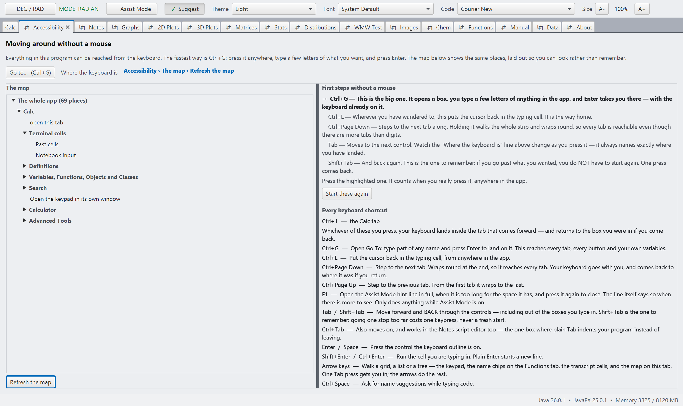
The Accessibility tab, showing the map of the program as a tree, the line naming where the keyboard is, and the shortcut list

Anywhere in the program, in about six keys

Press Ctrl+G from any tab, type a few letters of what you want (a button, a tab, or one of your own variables), and press Enter. The keyboard focus moves to that item, ready to use. Measured across the whole program, nothing is more than fourteen keys away, and most things are five or six. The arrow keys move through the matches and stop at the ends, and Esc closes the box and returns you to where you were, so opening it never costs you your place.

The keyboard focus travels with you. However you arrive at a tab (by a number shortcut, by Ctrl+Page Up or Page Down, from a search result, from the Help link on an error message, or by clicking the tab strip), the keyboard focus is placed inside that tab, ready to carry on. If you look at another tab and come back, you are returned to the exact box you were typing in.

A typeface chosen for readers

Atkinson Hyperlegible was thoughtfully designed by the Braille Institute to improve readability, especially for readers with low vision. It is built directly into the system so that every student sees the same clear, consistent typography regardless of their device. This page is set in it too, helping students focus their attention on the big ideas.

Text from 90% to 200%

If the text feels a little too small to read comfortably, simply press A+ a few times. Each press scales the entire system together, keeping headings proportionally larger than the body text so that everything remains clear, balanced, and easy to follow.

You can always see where you are

A clear, colored outline always shows which control has keyboard focus, so students never have to guess where they are. This support does not depend on knowing about Assist Mode—it is built into every interaction and remains visible across all fifteen themes. A student navigating entirely by keyboard should have the same confidence and sense of orientation as anyone else.

Assist Mode

With a single switch, the system becomes easier to see, understand, and navigate: buttons, pickers, and checkboxes become larger with more space around them; a bold outline clearly highlights whatever you point to; and a brief explanation appears to describe what each control does. The same information is also communicated to screen readers, so a student hears a meaningful name such as "power" rather than being left to interpret an unfamiliar symbol.

A reading aid for long numbers

For long whole numbers, a subtle grouping line is added beneath the digits to make the value easier to read at a glance. For example, 6 402 373 705 728 000 can be visually understood without changing the actual number. When copied, the value remains the plain sequence of digits, preserving its accuracy. The grouping uses thin spaces rather than commas because, in this language, 1,234 represents two separate values rather than a single large number.

Errors that teach

When something goes wrong, the system responds with a clear message in [square brackets], accompanied by a Help link that takes you directly to the relevant section of the manual. A mistake should not feel like a dead end or a failure. It should be an opportunity to understand what happened, learn from it, and move forward with greater confidence.

Color is never asked to work alone

Color is never expected to carry meaning by itself. A status is communicated through both color and a clear check or cross symbol, while graph curves are distinguished by dash patterns as well as hue. This thoughtful redundancy helps ensure that the meaning remains clear for students with color-vision differences and even when the work is printed in black and white. There are fifteen color schemes, four of them built for color-vision differences.

Everything is reachable by keyboard

Keyboard navigation is designed to be predictable and efficient. Ctrl + a digit takes you directly to a tab, and because there are sixteen tabs and only ten digits, Ctrl + Page Up and Ctrl + Page Down step along the whole row and wrap round at the ends, so every tab is reachable from every other one. If the row is too wide for the window, press anywhere on it and drag sideways; a plain click still selects the tab you clicked. Within the terminal, every cell can be reached using the arrow keys.

Tab takes you out of a box rather than typing a character into it — out of a cell, out of a graph expression row, out of the data boxes on the Stats tabs — and nothing you have typed is disturbed on the way. The one deliberate exception is the Notes script editor, where Tab indents your program because that is what you want there; Ctrl + Tab leaves any box at all.

We have also set a concrete accessibility goal: no tab should require more than 80 Tab-key presses to move through completely. That limit is measured and tested as in a science experiment, and the build fails if a tab exceeds it.

Undo, for the moment it matters

Restore last change provides a simple way to recover a definition that was accidentally overwritten or cleared, and if you attempt to close the window while work is only partly entered, the system pauses to ask before closing. These safeguards are intentional: they minimize unnecessary frustration and protect students from losing work. The goal is for productive struggle to occur where it belongs—in understanding the mathematics and the algorithms and developing new ideas—not in trying to navigate or recover from the system itself.

Assist Mode, seen rather than described

Here is the system with Assist Mode switched on. Nothing is hidden, removed, or rearranged—the structure and functionality remain exactly the same. It is the same learning environment, simply adapted to meet the needs of the student using it.

The switch is the second control along the top bar, so it is one click away and one click back. The controls grow and take more room around them, and the line across the bottom of the window explains whatever you are pointing at. In this picture it explains what Save Workspace does.
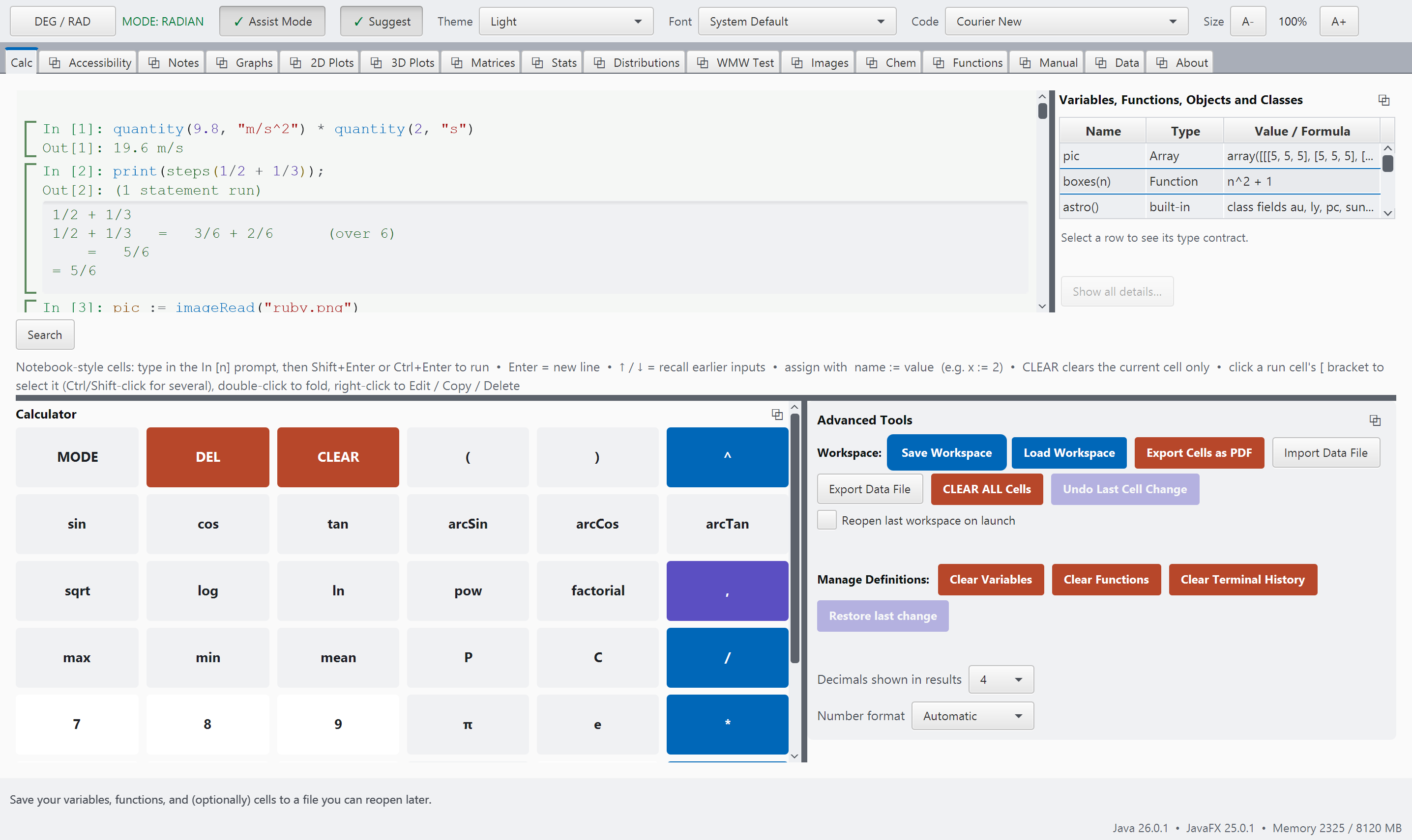
The system with Assist Mode switched on: larger keypad buttons with more space around them, and an explanation of the pointed-at control along the bottom of the window

Text size is a separate switch

Text size and Assist Mode are independent settings, because the students who need one are not always the students who need the other. This picture shows the ordinary system at 130% (three presses of A+) with Assist Mode off. Only the type has changed size. The same cells, the same panel and the same keypad are laid out again to fit. The setting is remembered, so a student who needs it sets it once.
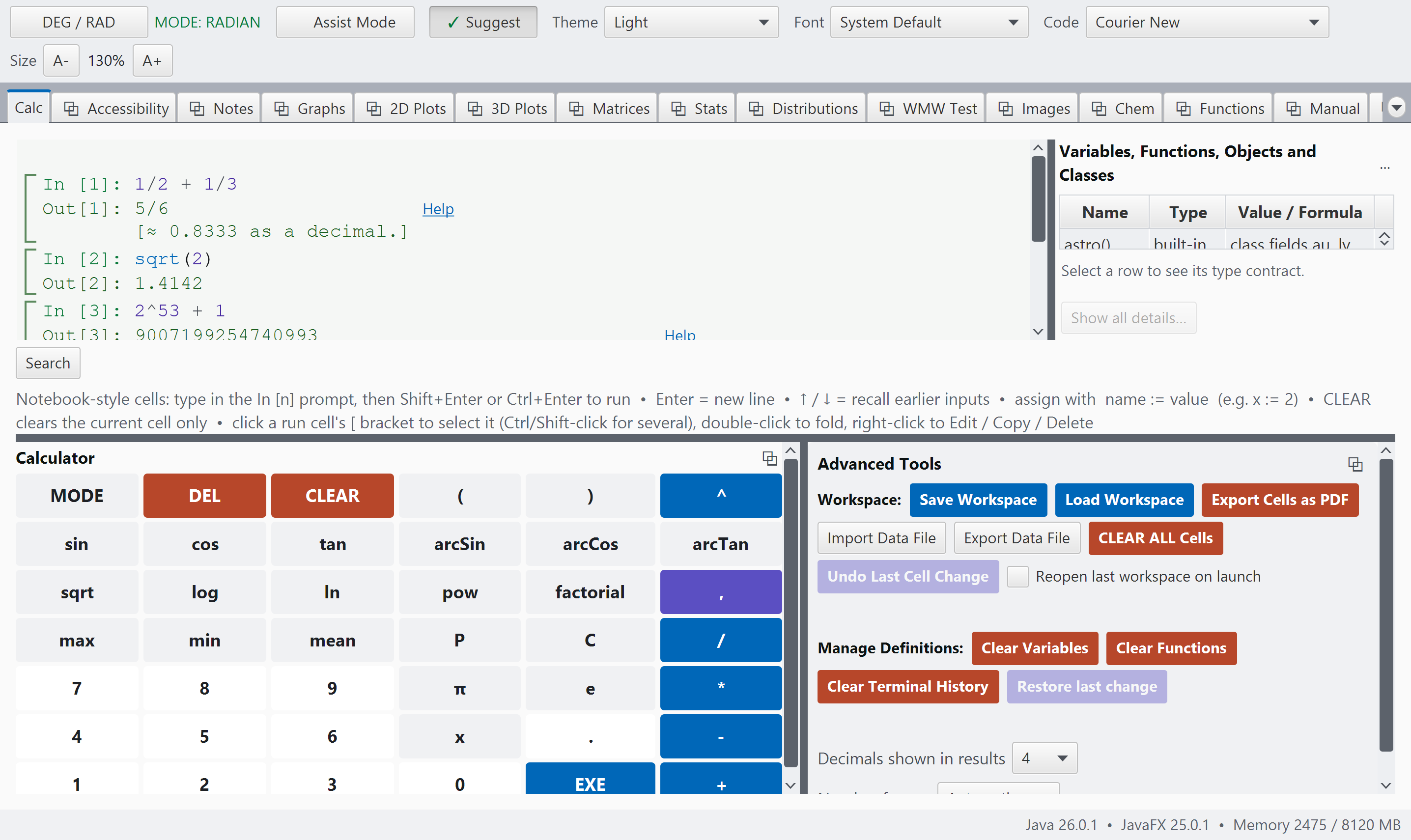
The same system at 130 percent text size, with Assist Mode off: the transcript, variables panel and keypad all re-laid out around the larger type

The Srivus language

Computational thinking reimagined

What you learn here, you take with you.

It seems to me to be a waste of effort, and a clear missed opportunity, that the time a student invests in learning a particular scientific calculator does not usually make learning a new programming language like R, Java or Python any easier afterwards. That is the gap this system intends to fill. Srivus shares many language structures with Java and Python, so the habits you build here are the habits you will need next.

Write your own functions

You can name a formula once and use it everywhere, in the calculator or on a graph. A quadratic expression is simply defined as f(x) := x^2 . There are advanced features such as lambdas and higher-order functions.

Real control structures

Blocks, if and else, while, for-in, C-style for loops, break and continue, and a switch with arrow arms and no fall-through. These are the same structures you will meet again in Java and Python.

Types you design yourself

Objects and classes, with private fields, constructors, methods, single inheritance and operator methods. As you dig deeper you will meet procedural programming, functional programming and object-orientation, and simple data structures such as lists, dictionaries, matrices, and tensors.

Checking your own work

The expect command encourages students to put their mathematical thinking into words by stating what they believe should happen and then allowing the system to check that expectation.

The spy command goes a step further by showing a value together with the expression that produced it, helping students connect results back to their reasoning.

Because the arithmetic is exact, == is exact too, and it says so plainly: 0.1 + 0.2 == 0.3 gives 0, since binary storage really does leave those two a hair apart. When a hair does not matter, as with a square root squared, a long sum, or a value that should have been zero, approx is the tolerant twin that asks the question you meant. It answers 1 or 0 and never stops the cell.

Reflective problem solving

Testing one's reasoning through codes is therefore introduced as a natural part of everyday reflective problem-solving rather than something reserved for advanced programming. The goal is to help students develop the habit of checking, questioning, and understanding their work from the very beginning.

And it compiles itself

A function may begin by being interpreted quietly, but after it has been used for roughly a third of a second, the system can automatically turn it into efficient compiled code. Students do not need to write anything, change their answers, or even think about the process—it happens behind the scenes without altering a single digit of their results.

For students who are curious about how the system works, the compiled version can be requested and explored by name. For everyone else, the experience is simply that their work becomes faster and more responsive as they use it.

In[x for x in range(1, 11) if mod(x, 2) == 0]
Out[2, 4, 6, 8, 10]

A list comprehension builds a new list and keeps only the values that pass the test. In other words, it is a list of all those x values 1 through 10 that are even, i.e., divisible by 2.
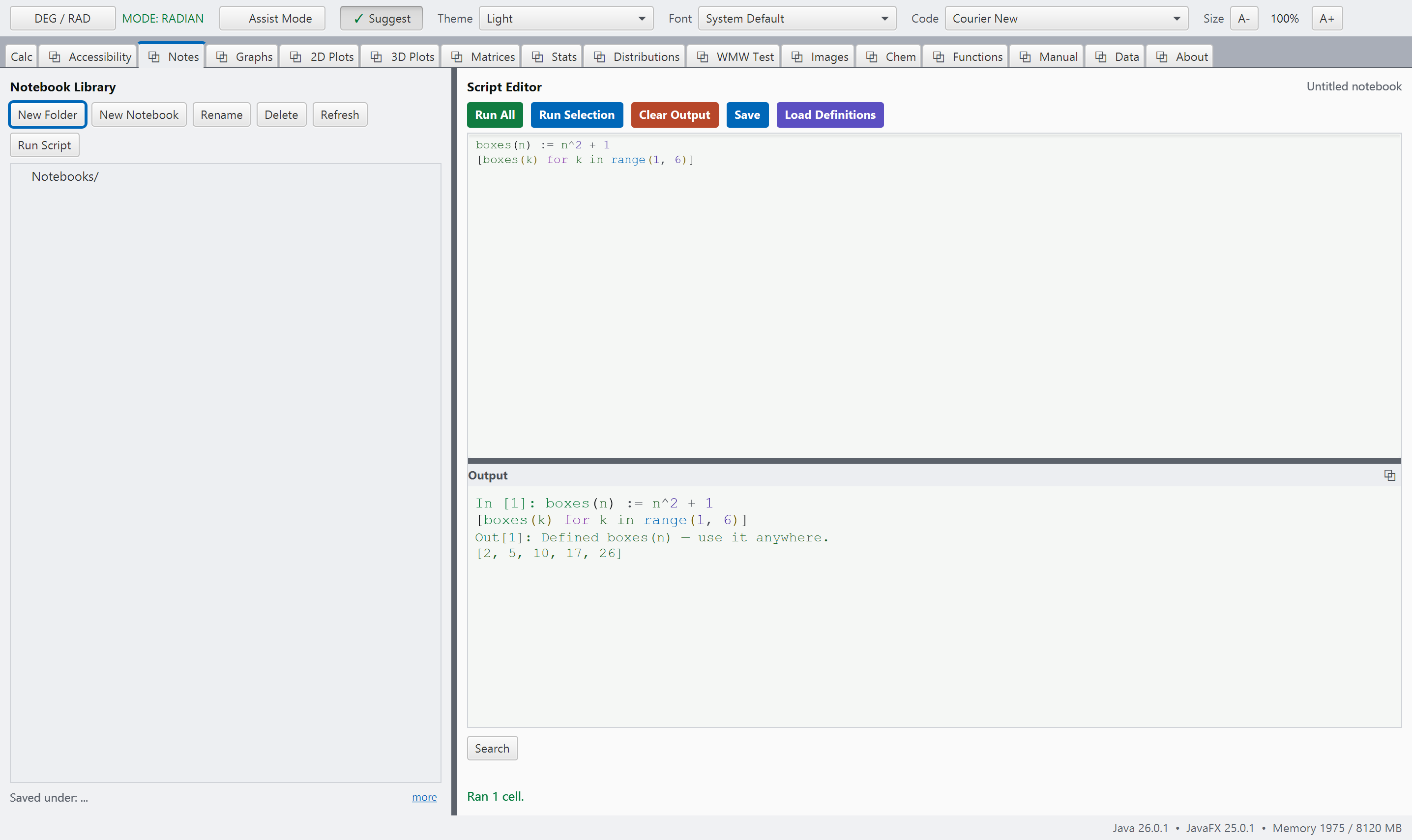
The Notes tab with a small program and its output
The Images tab: a photograph turned to ink lines by a two-step recipe, with the expression that produced it printed underneath and a histogram of the result below the picture
A picture is a value like any other, and nothing here is hidden from you: build the look with the sliders, and the Expression box underneath shows the call that produced it — imageXDoG(rgbToGray(pic), 1, 40, 30, 0.05) — ready to copy into a cell and keep.

Not only the answer

A calculator that can show its working

The working, i.e., the steps between the question and the answer, is what a student is graded on, and it is what a calculator usually hides.

Ask any calculator for one half plus one third and it gives 0.8333. The exercise, however, was about finding the common denominator. Therefore, this system keeps exact fractions as fractions, and steps() returns the working that produced them, written the way a student is asked to write it.

The steps shown are the real ones. steps() records the same computation that produces the answer, so the last line of a trace is always what the bare expression itself would have given. When there is no written work to show (a decimal calculation has none), the trace reports that there is none.

In both editions

Exact fractions, row reduction and long division

Three kinds of calculation produce a written method: exact fraction arithmetic, row reduction, and polynomial long division. Row reduction names each operation the way a textbook does, e.g., R2 - 1*R1, and the grid stays exact at every stage. Long division shows one trial term at a time.

Inprint(steps(1/2 + 1/3));
1/2 + 1/3 1/2 + 1/3 = 3/6 + 2/6 (over 6) = 5/6 = 5/6

The trace is text, and print writes its lines out as shown. The first line says what is being traced, the middle lines are the working, and the last line is the answer a bare expression would have given. Note that 1/3 is exactly one third (it is never rounded to 0.3333), and it stays exactly one third through every calculation it enters.

IntoFraction(0.375)
Out3/8

The conversion also goes the other way, so a decimal from a table can be turned back into the fraction the lesson is about.

A calculator session showing a steps() trace of exact fraction arithmetic, with the common denominator line visible
In both editions

Quantities carry their units

A quantity carries its unit. Every quantity is converted to SI units when it is entered and stays in SI units, so the discipline taught in a physics classroom (convert in, compute, convert out) is built into the arithmetic. Multiplying and dividing combine the units for you, like quantities cancel to a plain number, and adding meters to seconds gives an error message instead of a meaningless number.

Inquantity(20, "N") * quantity(3, "m")
Out60 J
Inquantity(3, "m") + quantity(2, "ft")
Out3.6096 m

Force times distance is energy, and the unit is worked out for you. Feet and meters add because they measure the same thing. The conversion is exact, so two feet is stored as exactly 381/625 m even though the answer line shows the decimal.

Temperature is handled with extra care, since 0 °C is 273.15 K. A temperature reading is a point on the scale and a temperature change is a difference between two points, and they follow the algebra a thermometer teaches: two readings subtract to give a change, and a reading plus a change is a reading. Two readings are never added, and a reading is never multiplied by a number.

Inquantity(30, "degC") - quantity(20, "degC")
Out10 K difference

The answer is ten kelvin of difference, and the word difference is part of the answer. A calculator that does not make this distinction produces a wrong physics answer without any warning.

The system stays out of the way

The system looks after your work.

A student's effort should go into the mathematics. It should not be spent on finding the line they wrote twenty minutes ago, on retyping a list they cannot reach, or on recovering an afternoon's work after a laptop lid closed. Everything in this section is in the free edition too.

In both editions

One search box for six places

One search box searches your own cells, the Functions reference, the Manual, the Data tab, a file you name, and a folder with everything under it. You tick which of the six places to search, and the results list which places were searched as well as what was found. The results panel has a border you can drag to give it more or less room, and it can be pulled out into a window of its own so that it sits beside your work.

None of this needs a mouse: type two characters, press Down to move through the results, and press Enter to go to one.

The search panel open under the terminal, with results from more than one source and the Where box showing which places are ticked
In both editions

Any panel can be moved into a window of its own

A small button in each panel's header (two overlapping squares) opens that panel in a window of its own. This works for the keypad, the Advanced Tools, the list of everything you have defined, the search results, the periodic table's trend plot, and any whole tab. Move the window to the side, or onto a second screen if you have one, and the space it leaves behind is given to the panels next to it.

Close that window and the panel goes back to where it was, at the width it was. In this way, a student who wants to compare a graph with the calculator can see both at once.

The calculator keypad floating in a window of its own beside the main window, whose remaining panels have spread to fill the space it left

If the power goes out

The system keeps a recovery copy of your session and rewrites it as you work. The copy is deleted every time you close the program properly. Therefore, if it is still there when you next start up, the program did not close properly, and you are offered your work back. On a normal day you never see it.

Reach back without retyping

ans is the previous answer. out(n) is the answer from any cell still on screen, referred to by the number printed beside it. The answer comes back whole, so a list is still a list and a matrix is still a matrix.

In[10, 20, 30]
Out[10, 20, 30]
Insum(out(3))
Out60

The list above was cell 3, so out(3) is that list again, with no retyping and no rounding.

A misspelled name gets a suggestion

Type a name that does not exist and the message suggests one that does, e.g., “Did you mean length?” A suggestion is offered only when the suggested name exists, so following it always works.

When the fix is a missing character, the message gives the whole line rewritten. Multiplication is never implied in this language, so (x+1)(x-1)/(x-1) is answered with “Missing multiplication sign? Write (x+1)*(x-1)/(x-1) — multiplication is never implied here.” The corrected line is there to be typed.

Drag a file onto the window

Drop a file on the program and it is filed in the folder where it belongs, with no dialog to work through. The status line then names the function that opens it, or tells you that there is no built-in opener for that kind of file.

One step back

Restore last change brings back a definition that was overwritten, cleared or deleted by accident, and a cell edit can be undone the same way. If you close the window with work only half entered, the program asks first.

Your work is a file you own

A workspace is saved to your own disk and opens in either edition. Cells can be exported as a PDF, and data comes in and goes out as files. None of it is sent to a server, since there is no server. See the privacy policy.

The editor suggests the name and how to call it

Type two letters and a list of matching names appears, each with its calling form, e.g., arcTan2(y, x). In this way, a student learns what a function takes while typing it. Your own variables and functions are listed first, above the built-in ones. After a dot, the list narrows to the functions that apply to the value in front of it. The calling forms come from the same reference the Functions tab prints, so the two never disagree.

A cell with ar typed into it and the completion list open, showing arcCos, arcCosh, arcSin, arcSinh, arcTan, arcTan2, arcTanh and arg, each with its calling form
After two letters are typed, every arc- name is listed with what it takes: arcTan(x), arcTan2(y, x), arg(z). Move through the list with the arrow keys.
A cell reading sqirt(2), answered by a message in square brackets naming the misspelling, saying capitals matter, and asking whether sqrt was meant, with a Help link beside it
When a name is wrong, the message says what was typed, why it failed and what to try instead, and it carries a Help link into the manual. Compare this with the single word ERROR that a hand-held calculator prints.

Srivus Plots

For when y = f(x) is not the shape of the answer.

Physics, chemistry and engineering courses ask for pictures that are not graphs of y = f(x): a rose curve, a trajectory, a field of arrows, a surface with its contours on the floor beneath it, the field lines of a magnet, a p orbital. Two tabs draw them.

Advanced Edition

2D Plots: one row is one plot

A pull-down at the left of each row sets the kind of plot, and each row has its own color, line style, sample count and range, and its own arrow and marker sizes. A polar row takes r as a function of theta, e.g., cos(3*theta) is a three-petaled rose, and the angle is read in whatever mode the DEG / RAD button is in. A parametric row takes a pair such as [cos(3*t), sin(2*t)]. A data row takes points, with error bars or as bars. An ordinary y = f(x) row can be put on logarithmic axes, one or both.

The other five kinds draw a whole plane from the same box. Density maps show z as color, contour maps draw its level curves, and vector fields draw the arrows, or the streamlines through them. Each streamline is followed until it leaves the window, arrives where the field vanishes, or returns to where it began. Slope fields draw the slope marks, and a phase portrait traces trajectories together with their nullclines. On a slope field or a phase portrait, type a starting point into the row and press Add to draw the solution through it. Alternatively, tick Click adds a solution, and every click on the plot starts a solution at the point you clicked.

Everything the free Graphs tab has is here as well: Trace, zoom and pan, a legend, axis labels, equal aspect, and saving the plot as a PNG. Auto-fit chooses a window that shows every visible row, and that is how both curves came to fit in the picture beside this. Sliders are shared across all three plotting tabs, so a slider named a drives every a you have written.

The 2D Plots tab with two rows drawn on one polar grid: a solid three-petaled rose from cos(3*theta), and a dashed Lissajous curve from the parametric pair cos(3t), sin(2t)
Two rows of different kinds, drawn in one window. The rose is polar, the dashed curve is parametric, and the legend names each row by the expression you typed.
Advanced Edition

3D Plots, and you can turn the picture round

Surfaces z = f(x, y) are the first row kind, colored by height with a scale beside them. Parametric surfaces take three expressions in u and v. A sphere or a torus is drawn this way. A solid of revolution spins y = f(x) about the axis, so the volume a calculus class integrates can be seen on screen. A space curve takes a triple in t, e.g., [cos(t), sin(t), t/4] is a helix. Implicit surfaces are written as an expression that equals zero on the surface, e.g., x^2 + y^2 + z^2 - 1 is the unit sphere. This is how you draw a shape that cannot be solved for z. Finally, plain data points in space can be plotted.

Two kinds are there for chemistry and physics. An orbital row takes a wavefunction, e.g., z*exp(-r/2) is a 2p orbital (in this row, r is the distance from the origin). It draws the surface inside which the electron spends most of its time, in one color where the wavefunction is positive and in another where it is negative, since bonding depends on the sign. Tick Cut away and choose the Front preset to see the nodes inside a 2s or a 3p orbital as the textbook draws them, or draw the same orbital as an electron cloud. The Examples menu carries the hydrogen orbitals from 1s to 4f. A three-dimensional vector field [P, Q, R] fills the box with arrows, and a point typed at the end of the row is followed both ways along the field line through it. Stream tubes draw those field lines as solid tubes, seeded around the center for you. This is the picture of a magnet found in every physics textbook, and the Examples menu has a dipole, a bar magnet, a straight wire, two wires, and Earth's tilted field.

Drag the picture to turn it, scroll to zoom, or use the Left / Right / Up / Down buttons and the arrow keys. There are camera presets, a perspective switch, and a Walk mode. A surface can be drawn filled, as a wireframe, as both, or smooth with no mesh showing. It can be made see-through, or drawn with its contours on the floor of the box beneath it. The picture shows the latter: the same function read as a surface and as its level curves at once. Lighting shades the whole picture, and you choose the direction of the light and the strength of the shading. Right-click saves the picture as a PNG, as everywhere else in the program.

The picture is drawn by the program itself and does not depend on the graphics card. Therefore, it works the same on a fifteen-year-old laptop in a computer lab as on a new machine.

The 3D Plots tab showing the surface sin(x) times cos(y) in perspective, colored by height with its color scale beside it, and the same function's contour lines drawn on the floor of the box underneath
One function, read two ways. The surface is sin(x)*cos(y), and the rings on the floor are its level curves, drawn from the same row.
The 3D Plots tab drawing the 3d z-squared hydrogen orbital as the surface enclosing 90 percent of the electron's probability: two lobes along the z axis in the row's blue, and a ring around the waist in the orange phase color
An orbital. The 3dz2 hydrogen orbital is drawn as the surface enclosing 90% of the electron's probability. The two lobes along z have one sign of the wavefunction, and the ring around the waist has the other. The row is (3*z^2 - r^2)*exp(-r/3), taken from the Examples menu.
The 3D Plots tab drawing a bar magnet's field as stream tubes: the tubes loop from the north pole at z = 1 round to the south pole at z = -1, colored by the strength of the field from purple far out to yellow at the poles, with a logarithmic colorbar beside the box
A magnet. A north pole sits at z = 1 and a south pole at z = −1, and the field lines are drawn as tubes that leave one pole and enter the other, seeded around the center by the tab. Color by magnitude paints each tube by the strength of the field along it, on a logarithmic scale, since a magnet's field falls off as a power of the distance.

Srivus Stats

Statistical thinking, made visible and meaningful

Abstract ideas become patterns you can see, explore, question, and understand.

In AP Statistics, the traditional use of printed statistical tables is really a legacy of an earlier era, when calculators and computers could not provide the precision and flexibility we have today. Tables were a practical solution to the limitations of the time, requiring students to work with a small set of rounded values rather than the underlying probability distribution itself. Today, we can move beyond that constraint. By working directly with a statistical plot, students can see significance levels, critical regions, and cumulative probability functions as parts of the same mathematical picture. Instead of searching for a rounded value in a table, they can explore the distribution, observe how probabilities change, and understand why a particular result is significant. The goal is not simply to replace a table with a graph. It is to replace a lookup procedure with understanding—using the greater precision and computational power available today to make statistical reasoning more visible, intuitive, and meaningful.

The Distributions tab, showing the standard normal density with the critical-value line at 1.6449, the left area shaded to 0.95 and the right tail shaded to 0.05
Distributions. Drag the critical-value line and the two shaded areas follow it, always adding to 1. This is the picture behind standardNormalInverseCDF(0.95), the 1.6449 an AP Statistics student meets first.
The Stats tab, showing a linear regression with its summary statistics and a scatterplot with the best-fit line
Stats. A regression and its one-variable summary, with the fitted line drawn under them.

The tab is in the Advanced Edition, but the statistical distribution functions are in both. chiSquareValue(10, 0.01) works in a cell in the free Basic Edition too.

Srivus Chem

The central science should have a place in every scientific calculator.

A printed periodic table offers one fixed perspective, and once it goes on the wall, that is the view students see all year. I wanted something more—a scientific instrument to explore, not simply a chart to reference.

So I built a periodic table with fifteen perspectives on the same 118 elements. From one simple menu, students can move among Atomic Mass, Electron Configuration, Oxidation States, Atomic Radius, Density, Electronegativity, and more.

The result is a living map of the central science, connecting chemistry, physics, mathematics, and statistics. Instead of memorizing one fixed chart, students can change the question, change the perspective, and discover the patterns for themselves.

Every element opens a detailed view, and every property can be used in a cell

Clicking on any element opens a detailed view showing all fourteen of its properties. More importantly, each of those properties can also be accessed directly from a calculator cell and used in a student’s own expressions.

That connection is especially important to me. I did not want the periodic table to be a separate picture of chemistry sitting beside the mathematics. I wanted the chemistry data to be part of the same system, so students can explore it, calculate with it, and make connections between scientific information and mathematical reasoning directly within the calculator.

InmolarMass("CO")
Out28.01
InmolarMass("Co")
Out58.9332

CO is carbon monoxide and Co is cobalt. One capital letter doubles the mass, and the calculator does not guess which you meant.

There is also a detachable trend plot under the table, so a property can be read across the whole table at once. Its axes carry real units, the pointer tells you which element it is over, and a mouse click pins a labeled card so that two or three elements can be compared side by side. The arrow keys do everything the mouse does.

The Chem tab showing the periodic table shaded by atomic mass
The detached trend plot, showing ionization energy against atomic number as a sawtooth, with the points colored by chemical family
The trend plot, detached. Ionization energy is plotted against atomic number, and the sawtooth pattern is periodicity itself.

It is readable in every theme

The shading is computed from whichever theme you are using, and it is held to the same contrast standard as the rest of the system, so the tiles carrying the largest values are always readable. Every tile also prints its own number, so the Grayscale theme, which has no color, loses no information.

The scale is chosen per property

The ratio of the maximum density to that of the minimum in the Chart is around 251,000. The plot of densities across the Atomic Mass cannot be drawn linearly. Therefore, it is drawn logarithmically. The legend always says which scale you are looking at.

The tab is in the Advanced Edition, but the chemistry data is in both. element("gold")["meltingpoint"], molarMass("H2O") and the whole chem.elements table work in a cell in the free Basic Edition too.

Data tab

Reference values, each one click from the expression that produces it.

A tab of curated scientific reference values. It is free in both editions, like the chemistry data beside it.

Eleven pages: the SI base and derived units and the seven defining constants, the SI prefixes, the Greek alphabet, conversion factors, a page of formulas, and then Physics, Chemistry, Biology, Astronomy & Cosmology, and Earth Science & Geology. A search box at the top takes you to the row that holds the answer.

In both editions

Click a value to copy the expression that produces it

Click a row (or Tab to it and press Enter), and the expression that produces the number is placed on your clipboard, ready to paste into a cell and calculate with. Larger entries, namely the planets, the moons, the star classes, the Sun, water and air, are shown as tiles. Open one and every value inside it copies the same way.

What is shown and what is copied always agree, since a displayed value is computed through the same path as the expression and formatted by the same formatter a cell uses. A reference table whose printed number differs from the number you get when you use it would be worse than no table at all.

Inplanet("earth")["escapeVelocity"]
Out11.19
Inmoon("Europa")["parent"]
Out"Jupiter"

The tab is one way of finding these values, and the language is where they are used. A student who never opens the tab can still type them, and a student who never types can still read the tab.

The Formulas page takes the same idea one step further: every formula on it is also a calculation. Click the row, paste the expression into a cell, change the numbers, and it gives the answer.

The Data tab, with a page of constants showing and one planet tile open as a pop-up listing its values

Typed in, answered back

Every example here has been run and tested.

These are not merely illustrations; they are carefully verified examples drawn directly from the system’s own reference. Every example is automatically tested, and the build will stop if even one result has changed unexpectedly. That gives us something important as teachers and scientists: a reliable connection between what we see in the manual and what the system actually does. When an example is included here, you can trust that it has been tested and works as described.

Complex numbers, everywhere

Ineig([[0, -1], [1, 0]])["values"]
Out[I, -I]

A quarter-turn rotation leaves no direction pointing where it started, so its eigenvalues cannot be real.

Matrices are just brackets

Insolve([[1, 1], [1, -1]], [5, 1])
Out[3, 2]

Two simultaneous equations are solved as a linear system. There is no special matrix type to learn first.

Statistics you can type anywhere

InstandardDeviation(2, 4, 4, 4, 5, 5, 7, 9)
Out2.1381

This is the sample standard deviation, which divides by n-1. The same call also accepts a single list.

The periodic table is built in

InmolarMass("Fe2(SO4)3")
Out399.878

Nested parentheses are read correctly, and the capitals carry meaning: CO is carbon monoxide, while Co is cobalt.

Chemistry as ordinary code

Inmap(el -> el["symbol"], filter(el -> el["standardstate"] == "Liquid", values(chem.elements)))
Out["Br", "Hg"]

Which elements are liquid at room temperature? Because the periodic table is a dictionary, ordinary list vocabulary answers a real chemistry question.

Say what you believe

Inexpect(1/3 + 1/3 + 1/3, 1)
Out"pass — 1, as expected."

A third three times really is one here, because two fractions are compared as the numbers they are rather than as the decimals they would round to. This is a student's first taste of writing a test.

Exact by default, tolerant when you ask

In0.1 + 0.2 == 0.3
Out0
Inapprox(0.1 + 0.2, 0.3)
Out1

Comparison is exact, so the classic decimal trap answers 0 rather than pretending otherwise: binary storage really does leave those two a hair apart. approx is the tolerant twin, for a number that came out of arithmetic rather than off a keyboard.

The functions a physics course runs into

InbesselY(0, 1)
Out0.0883

This is the Bessel function of the second kind, which is finite everywhere except at the origin, where it diverges.

A matrix in an exponent

InmatrixExponential([[2, 0], [0, -3]])
Out[[7.3891, 0], [0, 0.0498]]

For a diagonal matrix, each entry becomes e raised to that entry. This is a case you can check by hand before trusting the ones you cannot.

The last two examples are recent additions, and they arrived with many others. The special functions are included in full: both kinds of Bessel function, the Airy pair, the error function and its relatives, the Fresnel and Dawson integrals, the exponential integrals, the Riemann zeta and Debye functions, Lambert W, digamma, the Voigt profile, the spherical harmonics, and the hypergeometric functions on which many of the others rest. Beside them are the matrix functions: matrixExponential, which, given a vector as well, acts on the vector without forming the matrix exponential itself; matrixLogarithm, its inverse; and matrixSquareRoot. Finally, random is a class with several members, so random.uniform(), random.integer(1, 6), random.choice(...) and random.shuffle(...) read the way you would say them, and every distribution the program knows can be sampled.

The Functions tab open at the Fourier and Signals page, showing the FFT card with its usage line, its written-out definition, and worked examples in colored code beneath each one
The Functions tab, where these functions are documented. There is one card per function, with a usage line for every way it can be called and, where there is one, the exact definition written out, followed by examples that the build runs, colored the way the editor colors what you type. The tab can be searched by name or by any word in a description.

Fifteen themes

Four of them are there for color vision differences.

These are not merely decorative choices. They are designed with the same care we would give any other scientific instrument or mathematical tool, because color should help us see the data—not become a barrier to understanding or gaining insight from it.

Three of the palettes are based on the Okabe–Ito color set, with the order of the data colors carefully arranged to remain distinguishable for people with red–green or blue–yellow color-vision deficiencies. A fourth palette removes hue altogether, allowing the data series to be distinguished through differences in lightness alone.

Just as importantly, every one of the fifteen palettes is continuously checked against Web Content Accessibility Guidelines (WCAG) on contrast requirements through automated testing. This means a theme cannot quietly drift into becoming difficult to read. The goal is simple: whether you are exploring a distribution, comparing data, or teaching a statistical concept, the visual design should support your thinking, preserve accessibility, and keep the evidence in the data clear.

Mission

Reimagining STEM Education: Advancing Equity Through Digital Access and Freedom

I know I am pushing against a powerful trend in today’s subscription-based software economy, where essential digital tools increasingly sit behind recurring payments, creating a quiet divide between those who can continually afford access and those who cannot. In education, that divide is especially difficult for me to accept.

Both editions are complete by themselves.

Both editions share the same underlying language, but they are thoughtfully designed to support different groups of students. In the free edition, students can work directly in the calculator with matrices, statistics, dictionaries, classes, and their own functions—all through the same language they are learning. The Advanced Edition builds on that underlying language by adding nine dedicated tabs that give these areas of mathematics and science their own focused workspace. The goal is not to change what students can learn, but to provide the level of structure and support that best fits how they learn and work.

Whether this is a struggle that I can ultimately win is not the point. What matters is the effort to bridge the gap—to keep essential and beneficial digital tools within reach of students and schools, so that technology expands opportunity rather than quietly dividing people into those who have access and those who do not.

Perpetual license as a common good.

A perpetual license for an educational software has something in common with what I view as the idea of a common good: something created or acquired for the benefit of a community, where its value grows through continued use and shared access. The important resource is not only the software itself, but the knowledge, habits, lessons, and confidence that accumulate around it. Teachers learn how to use it effectively; students build familiarity with it; curricula develop around its capabilities; and a school can preserve that investment across generations of learners.

The power of perpetual license for users

True control: You buy the version you want and keep it for years.

Cost savings: You pay once and save money over time.

Offline freedom: The system works even when the internet goes down.

Peace of mind: No recurring charges on your or your guardian's credit card each month.

Two editions

Basic Edition

Free

For fifth graders — or earlier, if they are sincerely interested and adventurous — and up to those taking Algebra 2 or Precalculus. Personal use.

  • The complete Srivus language
  • Calc, with the full keypad
  • Accessibility, second from the left: a map of the whole program, and the fastest way to reach any part of it without a mouse
  • Graphs, for curves, relations and shading
  • The Functions reference
  • The whole Manual, all fifty-seven chapters
  • The Data tab: reference constants, units, conversion factors and the planets, with every value one click from a runnable expression
  • All fifteen themes, and every accessibility feature
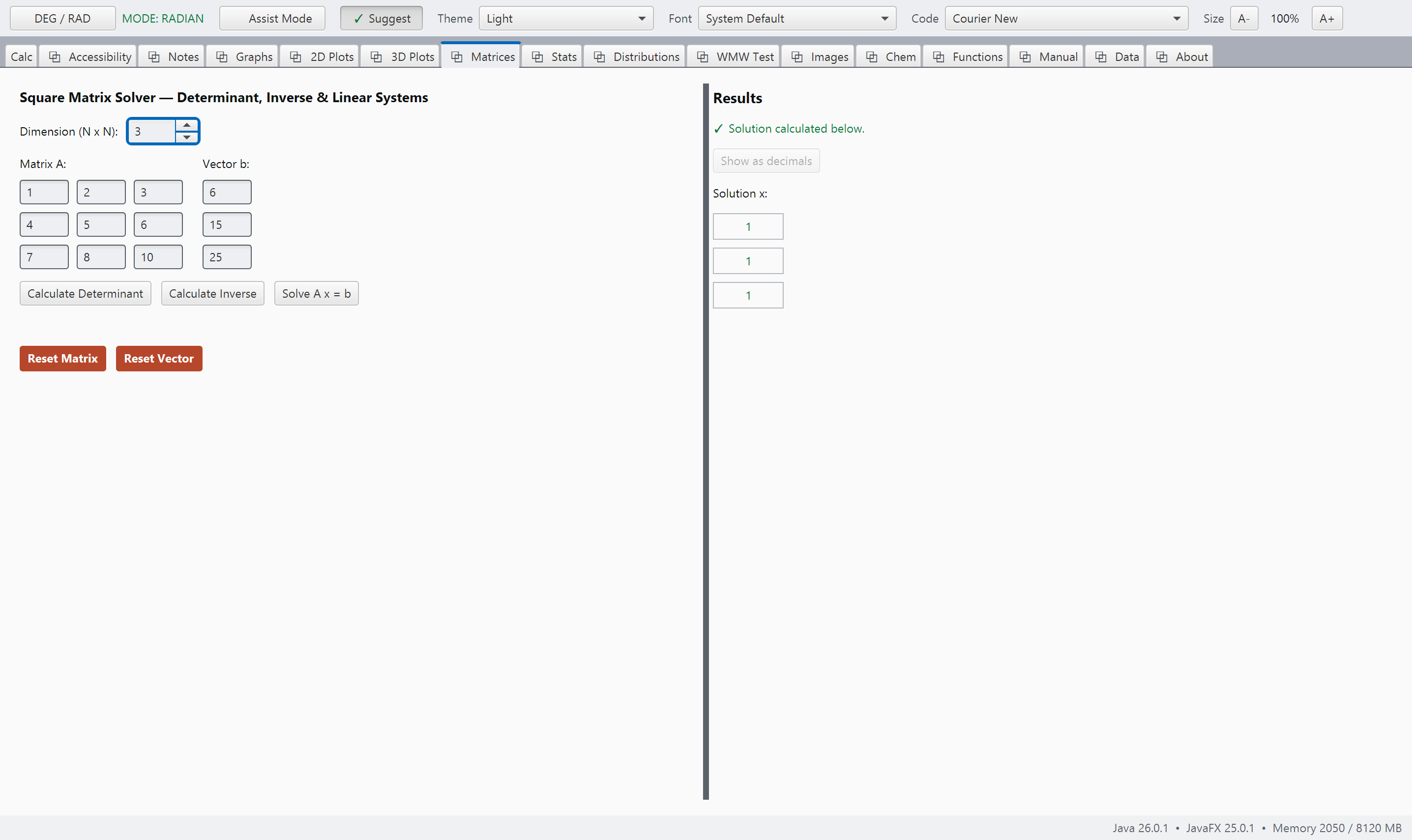
The Matrices tab, with a three by three matrix entered and its inverse shown beside it
The Matrices tab is one of the nine tabs the Advanced Edition adds. It gives a determinant, an inverse, or a solution to A x = b without your writing the call yourself. In the free edition, the same answers are one typed expression away.

For schools and districts

For a whole class, a school, or a district, let's get in touch only if you need the Advanced Edition.

The Basic Edition is free for your school as well as for your students. Please feel free to install it on as many school-managed devices as your students and teachers need, completely free of charge and without having to contact me for permission first.

For the Advanced Edition there is a site license, so that you are not buying seats one at a time, and it expressly allows your IT staff to install or image the software on school-managed devices for your students.

It also covers your students and staff at home. It is just as important to me that your students and staff can use it at home as they can at school. Your students and staff may install the software on a school computer or on their own personal one, because I believe learning should not stop when a student leaves the classroom. Based on my teaching experience at a high-need school, access to school devices was often not the greatest barrier—lack of wifi access at home was. A license that ended at the school gate would have missed one of the central purposes of building this system in the first place: giving students the opportunity to continue learning wherever they are.

They keep it after they leave. A student who graduates, transfers or moves on does not lose the software, and neither does a teacher who retires. It stays on their own computer permanently, whatever happens to the school's license afterwards. A tool that a student has learned to think with should not be taken away on the day they finish learning with you. If the license ended at graduation, it would be a rental with a long lease, and the purpose of this project is that students should not have to rent the tools they learn with.

The fact that the software runs completely offline is another part of that commitment to accessibility. In a computer lab, it does not require additional bandwidth, special filtering exceptions, or a separate sign-in process for every student. Everything stays on the local computer, so student information is not transmitted or collected at all. It aligns perfectly with the above-mentioned principle YDNB—“Your Data, Not My Business.”

Site license for the Advanced Edition

It is a single, perpetual license in one payment—there is nothing to renew and no annual subscription to remember or budget for again. Pricing is based on your school’s total enrollment, a number your school already knows, so there is no need to count devices, track licenses, or spend time managing hardware. The aim is to keep the decision simple with no endless recurring cost, allowing the focus to remain where it belongs: on supporting students and teachers.

Site license prices by school enrollment
Your schoolOne-time
Under 200 students$399
200 to 599 students$899
600 to 999 students$1,399
1,000 to 1,999 students$2,199
2,000 to 3,499 students$2,999
3,500 or more, or a whole districtfrom $4,500

Purchase orders are welcome, and you do not have to wait for me to start. Make yourself a quotation to attach to your requisition, and ask me for a W-9 or a sole source letter whenever your business office needs one.

If the price is the reason your school cannot have this, please write to me. I would genuinely rather see this software in your classroom than have cost be the reason your students cannot benefit from it. I have taught in a high-need school myself, so I understand firsthand how difficult budget conversations can be and how often limited resources force teachers to make painful choices. I want every student—regardless of their school’s budget—to have the opportunity to use great educational tools that can support their learning, including this software. Please reach out and I will make it work!

Create a quote for your school Or email me directly

Questions

The questions I hear first.

Does it need an internet connection?
No. It does not need the internet to install, to run, or at any point afterwards. The whole language, the manual and the full reference are on your machine. There is no account, there is nothing to sign in to, and nothing is ever sent anywhere.
What does it cost?
The Basic Edition is free. It is a complete calculator, it does not expire, and nothing in it is time-limited. The Basic Edition is free for the whole school too. The Advanced Edition is $39, paid once, with a perpetual license, so you buy it once and it stays with you. There is no subscription. For schools there are site licenses priced by enrollment, and the table is in the schools section of this page. If your school acquires the site license for the Advanced Edition, you also get to use the Advanced Edition on your own computer for free.
Which Java do I need?
You need Java 23 or newer. Java 25 is the current long-term-support release and is the easiest choice. Java 17 and 21 are very common downloads but they will not work, because the system is built against a version of JavaFX that requires Java 23, and on an older Java it stops before the window even appears. The download page walks you through step-by-step with the installation process specific to your operating system.
Is my work stored on someone else's computer?
No. Your files stay on your own machine. Nothing is uploaded anywhere, because there is nowhere for it to be uploaded to.
Will it run on a school Chromebook?

On ChromeOS, support depends on the hardware and on the school’s device-management policies. The application is distributed as a Java JAR file, so the Chromebook must have the Linux (Crostini) environment enabled and a compatible Java runtime available. Many school-managed Chromebooks disable Crostini entirely, in which case a JAR application cannot be run locally.

For Intel/AMD Chromebooks, the standard JAR download can generally be used once Linux and Java are available. ARM-based Chromebooks are not currently supported. On Windows, macOS, and Linux computers, the same JAR can be used with a compatible Java runtime, although the installation and file-association steps differ by operating system.

For school-managed devices, the practical advice is simple: talk with your school IT specialists to see if it can be installed. For IT personnel, please test the actual installation on one student device before deploying it broadly or planning classroom use. Verify the Java runtime, operating-system compatibility, application permissions, file associations, network and security policies, and any school device-management restrictions before approving the application for student use. A technically capable application is only useful in a classroom when the school’s hardware, operating system, Java runtime, and management policies all permit it to run.

What is the difference between the two editions?
The language is complete in both editions. The Advanced Edition adds nine dedicated tabs for older students, namely Notes, 2D Plots, 3D Plots, Matrices, Stats, Distributions, WMW Test, Images and Chem.
Can I use it with a whole class?
Yes. The Basic Edition is free for your school to install on as many managed devices as you like, and you do not need to ask me first. For the Advanced Edition there is a site license priced by your school's enrollment. It covers your students and staff at home as well as on school machines, and they keep it after they graduate or leave. The prices are in the schools section above. I will send an invoice, since schools rarely buy with a card.
How does a student learn it from a standing start?
The Manual inside the system is a reasonably complete course on its own. It opens with a Welcome page that lays out the route, then a short Start Here, and the chapter after that, First Steps — Four Tasks, Start to Finish, walks a beginner through storing an answer, writing their own function, shading a region on a graph, and saving their work. All four tasks work in the free edition.
Is the name Srivus, or Scientifica?
Both, the way a car has a make and a model. Srivus is my one-person business, and it is also the name of the calculator's programming language. Scientifica is the model name of this calculator system. On the label they read together: Srivus Scientifica.
Something looks wrong. What should I do?
Please write me a note. A worked example that gives the wrong answer, a message that does not explain itself, or a topic you needed and could not find are all important for me to know about, and suggestions are as welcome as bug reports. A short note saying what you typed and what came back is usually enough for me to act on.